Logistic Regression

10 mins read. Logistic Regression with a Neural Network mindset.

Logistic Regression

Logistic Regression is a statistical method used for binary classification. Despite its name, it is employed for predicting the probability of an instance belonging to a particular class. It models the relationship between input features and the log odds of the event occurring, where the event is typically represented by the binary outcome (0 or 1).

The output of logistic regression is transformed using the logistic function (sigmoid), which maps any real-valued number to a value between 0 and 1. This transformed value can be interpreted as the probability of the instance belonging to the positive class.

Sigmoid Function

Now we use the sigmoid function where the input will be z and we find the probability between 0 and 1. i.e. predicted y.

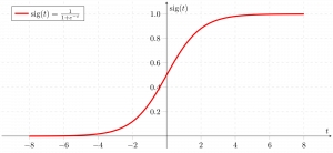
As shown above, the figure sigmoid function converts the continuous variable data into the probability i.e. between 0 and 1.

• 𝜎(𝑧) tends towards 1 as 𝑧→∞

• 𝜎(𝑧) tends towards 0 as 𝑧→−∞

• 𝜎(𝑧) is always bounded between 0 and 1

where the probability of being a class can be measured as:

𝑃(𝑦=1)=𝜎(𝑧)

𝑃(𝑦=0)=1−𝜎(𝑧)

def sigmoid(z):
    """
    Compute the sigmoid of z

    Arguments:
    z -- A scalar or numpy array of any size.

    Return:
    s -- sigmoid(z)
    """
    
    s = 1/(1+np.exp(-1*z))
    
    return s

Cost Function

A cost function is a mathematical function that calculates the difference between the target actual values (ground truth) and the values predicted by the model. A function that assesses a machine learning model’s performance also referred to as a loss function or objective function. Usually, the objective of a machine learning algorithm is to reduce the error or output of cost function.

Plotting this specific error function against the linear regression model’s weight parameters results in a convex shape. This convexity is important because it allows the Gradient Descent Algorithm to be used to optimize the function. Using this algorithm, we can locate the global minima on the graph and modify the model’s weights to systematically lower the error. In essence, it’s a means of optimizing the model to raise its accuracy in making predictions.

Log Loss for Logistic regression

Log loss is a classification evaluation metric that is used to compare different models which we build during the process of model development. It is considered one of the efficient metrics for evaluation purposes while dealing with the soft probabilities predicted by the model.

The log of corrected probabilities, in logistic regression, is obtained by taking the natural logarithm (base e) of the predicted probabilities.

Hence, The Log Loss can be summarized with the following formula:

where,

• m is the number of training examples

• is the true class label for the i-th example (either 0 or 1).

• is the predicted probability for the i-th example, as calculated by the logistic regression model.

• is the model parameters

In summary:

• Calculate predicted probabilities using the sigmoid function.

• Apply the natural logarithm to the corrected probabilities.

• Sum up and average the log values, then negate the result to get the Log Loss.

Forward and Backward propagation

Implement a function propagate() that computes the cost function and its gradient.

Forward Propagation:

• get X

• compute $A = \sigma(w^T X + b) = (a^{(1)}, a^{(2)}, ..., a^{(m-1)}, a^{(m)})$

• calculate the cost function: $J = -\frac{1}{m}\sum_{i=1}^{m}(y^{(i)}\log(a^{(i)})+(1-y^{(i)})\log(1-a^{(i)}))$

Here are the two formulas you will be using:

import numpy as np
from public_tests import *

def propagate(w, b, X, Y):
    """
    Implement the cost function and its gradient for the propagation explained above

    Arguments:
    w -- weights, a numpy array of size (num_px * num_px * 3, 1)
    b -- bias, a scalar
    X -- data of size (num_px * num_px * 3, number of examples)
    Y -- true "label" vector (containing 0 if non-cat, 1 if cat) of size (1, number of examples)

    Return:
    grads -- dictionary containing the gradients of the weights and bias
            (dw -- gradient of the loss with respect to w, thus same shape as w)
            (db -- gradient of the loss with respect to b, thus same shape as b)
    cost -- negative log-likelihood cost for logistic regression
    
    Tips:
    - Write your code step by step for the propagation. np.log(), np.dot()
    """
    
    m = X.shape[1]
    
    # FORWARD PROPAGATION (FROM X TO COST)
    Z = np.dot(w.T, X) + b
    A = 1/(1+np.exp(-1*(Z)))
    cost = (-1/m)*np.sum(Y * np.log(A) + (1-Y) * np.log(1-A))
    
    # BACKWARD PROPAGATION (TO FIND GRAD)
    dZ = A - Y
    dw = (1/m)*np.dot(X, dZ.T)
    db = (1/m)*np.sum(dZ)
    
    cost = np.squeeze(np.array(cost))
    
    grads = {"dw": dw,
             "db": db}
    
    return grads, cost

Reference

Logistic Regression in Machine Learning - GeeksforGeeksGeeksforGeeks

Cost function in Logistic Regression in Machine Learning - GeeksforGeeksGeeksforGeeks